|
The ambient problem ‘The Island is full of noises’, Shakespeare, The Tempest
By David Mawdsley, Managing Director, Laplace Instruments Ltd
Perhaps we should now write ‘The World is full of noises’. Certainly, from an electromagnetic point of view, you need only to glance at the plot from an RF spectrum analyser to see that we are living in a welter of man-made noise that threatens to overwhelm any measurements we might want to take in unscreened environments.
The issue of the effectiveness of ambient (background) noise cancellation has been long debated. However, there seems to be little published evidence to justify the claims made by either side of the debate. This paper is the result of some simple experiments that were performed by the author in an attempt to provide a clear answer to the question ‘Does ambient cancellation work?’. The conclusions were (at least to me) unexpected and surprisingly clear-cut!
There are two situations in which cancellation may be used; identification and measurement. Identification techniques are used to simply locate EUT emissions in the presence of high ambients. Those who have attempted to locate emissions reliably without some kind of ambient cancellation will know how frustrating this can be. Measurement techniques go one step further and are able (potentially) to measure the EUT emission levels with some degree of accuracy. This paper addresses this second, more demanding requirement.
Two approaches to the problem of ambient cancellation are currently on offer from EMC test equipment manufacturers…
1. To measure just the ambient first, then to take a second measurement with the EUT switched on and use software to subtract the first from the second measurement (difference technique).
2. To use a twin channel analyser that can either:
a. Correlate a near field probe input with the far field antenna input. The assumptions being that any significant emission must be detectable in the EUT near field and that near field probes are ‘blind’ to ambient signals.
b. Use two far field antennas, one at a significant distance from the test site, and use difference techniques to extract the EUT emissions.
Each technique has its pros and cons. None are perfect! For instance technique 1 suffers in the presence of fluctuating ambient (and ambients always fluctuate to some extent) but has the advantage of potentially being accessible to any standard EMC receiver or analyser. Both options 2 require the use of a specialist twin channel EMC analyser and 2(a) exposes as false the assumption that near field probes are immune to ambient. In reality, strong ambients are induced into any cabling associated with the EUT and re-radiated as a near field signal. Both 1 and 2(b) depend on the validity of the ‘difference’ technique, and it is this technique, which is the subject of this paper.
The validity of using some kind of ‘difference’ trace to calculate the emission levels from an EUT in the presence of ambient is based on the assumption that the field strength will increase when two or more sources are present. This seems obvious, and is confirmed by the behaviour of OATS sites. It is well known that the ground-reflected signal combines with the direct signal on a standard site to increase the field strength by almost 6dB, which on a linear scale is a x2 factor. Reasonable enough, given that the two signals will be of similar strength. Of course, the signals in this case are strictly coherent (from the same source) and are in phase. Changing the phase relationship (for instance, by varying the height of the antenna) will completely ‘undo’ this happy result. So phase matters. But does it matter when we are considering an EUT emission and an ambient signal? This is one of the aspects for investigation in the following experiments.
The Experiments We created a known ‘ambient’ and a known ‘EUT’ signal and studied how the field strength as measured by an EMC analyser was affected when both were on together. The type of signals to create were considered…
Signal types, broadband and/or narrowband?
Signals of both types are common, both from EUTs and in the ambient. We should not assume that any cancellation technique would work equally well (or badly) for all combinations of these two signal types.
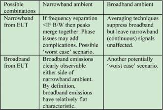
Table 1 shows the potential combinations with notes
It seems from the above that the toughest challenge for any cancellation techniques is when both EUT and ambient signals are of the same type of signal. Therefore our experiments modelled these two situations.
The Narrowband Experiment The test involved the use of two emissions reference sources (ERS) from Laplace Instruments Ltd, one to simulate the background (ambient) level, the other to simulate an EUT. These are ‘comb’ generators, essentially narrowband sources with a continuous (in time domain) emission output. They radiate a signal with 2MHz spacing and the two units have a very close frequency matching (actually within 40ppm), well within the resolution bandwidth of the analyser. Thus presenting an almost ‘worst case’ scenario. The close frequency matching prevents the use of frequency discrimination to separate the signals and the steady state nature of both prevents the use of averaging techniques.
The ERS units actually give very similar radiated output levels, but they were located in different positions in the test site (the laboratory) so that the signals received at the measurement antenna were different from each. The difference is due to the change in ‘site attenuation’ at the two locations.
The frequency range 350 - 450MHz was chosen, as this range was relatively free of other background signals.
Each ERS was initially measured separately. The one which gave the lowest levels (as measured by the antenna) was chosen to represent the EUT. This we called unit A. The other (unit B) then represented the ambient.
A sequence was then followed to represent a real EMC test…
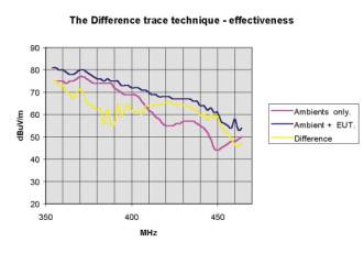
The first plot shows the ‘ambient only’ (unit B) spectrum and the increased level when the EUT is switched on, (units A and B)
The second plot shows the calculated difference trace. Note that this is NOT the simple difference (A-B) but one that takes the log scaling into account. This is the estimated level of the emissions from the EUT
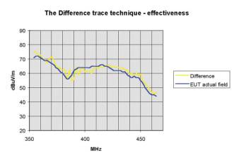
The third plot is a comparison of the estimated level and the actual level of emissions from the EUT. To calculate the signal which caused the field to rise from level XdBuV/m to level YdBuV/m we cannot simply subtract the to numbers to find the difference.
Subtracting two log values is the equivalent of dividing one by the other. So these values must be converted back to linear values first using the formula X(lin) = 10(X(log)/20) Then the difference Z(lin) = X(lin) – Y(lin). Finally, Z is converted back to log (dB) values. ZdBuV/m = 20log(Z(lin)).
As can be judged, the plot of estimated vs. actual shows excellent correlation. The fact that at 380MHz, the difference trace is within 4dB of the actual even though the EUT is over 15dB below the ambient level, shows that this technique can be remarkably effective.
This experiment has used two independent sources, hence the signals are incoherent. Incoherent signals are not phase locked. This will be the reality when dealing with EMC applications when an ambient signal is to be ‘cancelled’. A phase relationship will exist between the EUT and each ambient source, causing the combined field to fluctuate at the difference frequency. So a 253,456,789Hz ambient and a 253,456,800Hz EUT signal will mix to create a 211Hz resultant or fluctuation frequency. When using a QP detector with a band C time constant of 550msec, it is obvious that these fluctuations will not affect the resultant. Indeed, for any phase effect to be observed, the two frequencies will need to be within a couple of Hz, possible, but highly unlikely, especially over any meaningful period of time.
The only problem that would affect the results is that of an unstable ambient. A technique has been routinely used by the author and others to stabilise the ambient by using an averaging or max. hold technique when acquiring both the ambient trace and the ambient+EUT trace. Typically, using either technique on a set of 8 scans produces a stable result. The difference trace then produces a relatively ‘clean’ measure of the emissions from the EUT. Naturally, there is often some rogue transmission that is timed so as to appear as an EUT emission, but simple ‘common sense’ investigations soon real these as not originating from the EUT.
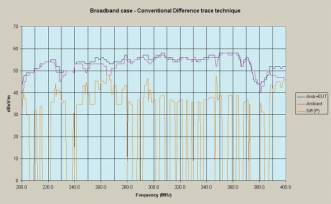
The Broadband Experiment The above procedure was repeated, but this time using two broadband sources, the York Electromagnetics CNE (Comparison Noise Emitters). These produce a relatively flat output spectrum with high bandwidth impulsive noise sources.
Again the emissions from each were plotted separately at first.
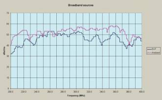
Then plots were taken with first one then both sources switched on. The plot shows the results. The difference trace includes intermittent excursions to minus infinity where the calculation attempts to find the log of zero! The cause of this little difficulty is at frequencies where the ambient result and the ambient + EUT result are the same (or negative).
The final plot shows the actual EUT level and the difference trace as calculated for the narrowband experiment (Orange trace). The results show that the technique has failed to provide even a rough estimate of the levels from the EUT. Clearly the signals were not interacting together in the same way as the narrowband sources. In an attempt to improve the result, the difference was recalculated using a voltage base (V) rather than a power base (V2). The magenta trace shows that whilst it is better, there are still wide inconsistencies.
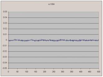
Use of the QP and Average detectors did not significantly improve matters. In an attempt to resolve why the two signals apparently did not ‘sum’ together, the signals from the receiving antenna were plotted in the time domain. The following 4 plots are all acquired on a fast digitising DSO (500MHz sampling rate). The time axis is in nanoseconds and the vertical scale is identical for all these plots.
Plot sc1004 shows the ambient as output from the log periodic antenna with no sources switched on.
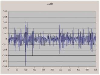
Plots sta002 and stb000 show the signal from the antenna with each source switched on independently. The impulsive nature of these sources is immediately evident. Fourier analysis shows that for a flat (ish) spectrum in the frequency domain, the time domain must have a transient nature. The signals are completely random in nature, as expected from noise sources.
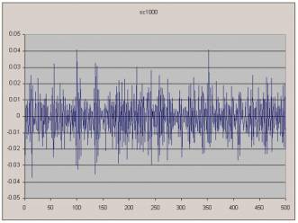
Plot sc1000 shows the two sources radiating simultaneously. The frequency of the impulsive spikes has increased, in fact doubled, but the peak levels are unaffected.
Thus a peak detector will generally maintain the same level as the strongest source, unaffected by the presence of any source with a lower level of impulsive peaks. This assumes that the spectral bands of the two sources overlap. If this were not the case, identification of the EUT emissions would be simple!
A calculation to show the level of signal in each waveform was undertaken by summing the absolute values of all the DSO samples in each frame.
Ambient only 0.3696V Source 1 3.7744V Source 2 3.6467V Both sources together 5.1472V
This shows that there is the expected increase in signal in the time domain.
It was thought initially that the use of an average or QP detector would improve the performance of the difference technique. This was not observed. Further thought regarding the average and QP detectors as specified by CISPR16 shows why. The output from these detectors is critically dependant on the repetition rate of the incoming impulses. Time constants within these detectors are such that for repetition rates above 10KHz, the detector output will be equal to that of a peak detector. In other words, once above 10KHz, increasing the repetition rate will have no effect. A study of the waveforms shows that significant impulses occur at a median interval of approximately 300nS, equivalent to a repetition rate of 3.3MHz. Well above 10KHz!
Clearly, the above analysis holds true for the noise sources we used (the CNEs). Other noise sources with different characteristics may behave differently. For instance, some sources of ‘real world’ noise are caused by mains frequency switching devices (such as phase angle controllers). These have an impulse repetition rate of 100Hz (or 120Hz). Doubling the rate by introducing a second source would increase the QP level by some 3dB and the average level by approximately 6dB. This suggests that a difference technique would work, but factors such as relative timing (ie relative phase angles) and duty cycle may influence the results.
Coping with the Real World Overall, this experiment has shown that in real world situations where both the background and the EUT emissions are broadband with overlapping spectra, and the nature of the noise sources is unknown, (this must be particularly true of the background), the use of any difference technique should be avoided where possible. In practice however, a modified difference trace technique has been successful in detecting the general spectrum of broadband emissions from an EUT, even in situations of high level ambient. This modified technique involves the use of an average scanning technique coupled with a peak detector.
1. With the EUT off, free run the analyser and calculate the average level at each frequency point over the several sweeps.
2. When the resultant has stabilised, cease scanning and store this as the background trace.
3. Switch the EUT on and repeat the average scanning process until the resultant has stabilised.
4. Plot the difference between the two results.
Although not recommended for accurate measurements, this technique does seem to give an excellent estimation of the EUT emissions for pre-compliance purposes.
Summary Where the ambient and EUT sources are of different signal types (narrowband and broadband) the measurement of EUT emissions is generally possible with common sense judgement.
The difference trace technique works well in the narrowband /narrowband situation, provided that the background is stable. However, additional techniques are available that have proved very effective in coping with unstable backgrounds.
When both ambient and EUT emissions are broadband, measurements become unreliable and the difference technique fails even to provide an approximation of EUT levels. However, the nature of the sources used in the experiment may not be typical of the real world. Experience has consistently shown that the difference trace technique does provide a useful guide for EUT emissions even in worst-case situations. This is probably due to the lower repetition rates (100s of Hz) that are typically causing the ‘real’ broadband emissions.
David Mawdsley can be contacted on +44 (0)1263 515160, tech@laplace.co.uk or visit http://www.laplaceinstruments.com/
|